Taylor Series

A Taylor series is an infinite sum that approximates a function using its derivatives at a point, helping express complex functions as simpler polynomials for analysis and calculation.

\[ f(x) = f(a) + f'(a)(x - a) + \frac{f''(a)(x - a)^2}{2!} + \frac{f'''(a)(x - a)^3}{3!} + \cdots \]

Import Libraries

import numpy as np
import matplotlib.pyplot as plt

Factorial

\[ x! = x \times (x-1) \times (x-2) \times \ldots \times 3 \times 2 \times 1 \]

def factorial(x):
    if x<=1:
        return 1
    else:
        product=1
        for i in range(1,x+1):
            product*=i
        return product

Defining Function

def function(x):
    return 1 + x + x**2 + x**3 + x**4

Setting up the variables

x=1     # Point where we like to approximate the value of fxn
a=0     # Value of x where we know about the fxn

Find nth derivative of a fxn at point a

def derivative(f, x, n):
    if n == 0:
        return f(x)
    else:
        h = 1e-2
        df = (derivative(f, x + h, n - 1) - derivative(f, x, n - 1)) / h
        return df

Exact Ans

exact=function(x)

Estimated Answers

def estimate(terms, a, x):
    sum = 0
    for i in range(terms):
        sum += derivative(function, a, i) * (x - a)**(i) / np.math.factorial(i)
    return sum

order = []
errors = []

print("Order\tExact\t\tEstimate\tError (%)")
print("-------------------------------------------------------")
for i in range(1, 11):
    estimate_ans = estimate(i, a, x)
    error = np.abs(exact-estimate_ans)/exact*100
    print(f"{i-1}\t{exact:.9f}\t{estimate_ans:.9f}\t{error:.9f}%")
    order.append(i-1)
    errors.append(error)

plt.figure(figsize=(5, 3))
plt.plot(order, errors, marker='o')
plt.xlabel("Order")
plt.ylabel("Error (%)")
plt.title("Error vs. Order")
plt.grid(True)
plt.show()

Order   Exact       Estimate    Error (%)
-------------------------------------------------------
0   5.000000000 1.000000000 80.000000000%
1   5.000000000 2.010101000 59.797980000%
2   5.000000000 3.040801000 39.183980000%
3   5.000000000 4.100801000 17.983980001%
4   5.000000000 5.100801002 2.016020044%
5   5.000000000 5.100800873 2.016017454%
6   5.000000000 5.100806732 2.016134644%
7   5.000000000 5.100599667 2.011993336%
8   5.000000000 5.106547290 2.130945803%
9   5.000000000 4.963363765 0.732724697%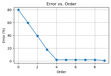

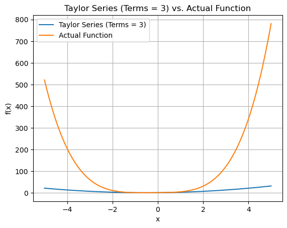
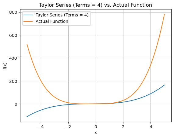
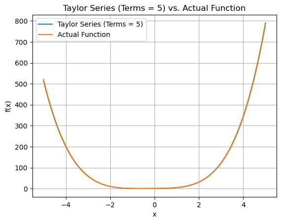
Plotting the Exact and Approx Functions

x_values = np.linspace(-5, 5, 400)
a = 0

for terms in range(2,6):
    plt.figure()
    approx_y_values = [estimate(terms, a, x) for x in x_values]
    plt.plot(x_values, approx_y_values, label=f'Taylor Series (Terms = {terms})')
    plt.plot(x_values, function(x_values), label='Actual Function')
    plt.title(f"Taylor Series (Terms = {terms}) vs. Actual Function")
    plt.xlabel("x")
    plt.ylabel("f(x)")
    plt.legend()
    plt.grid(True)
    plt.show()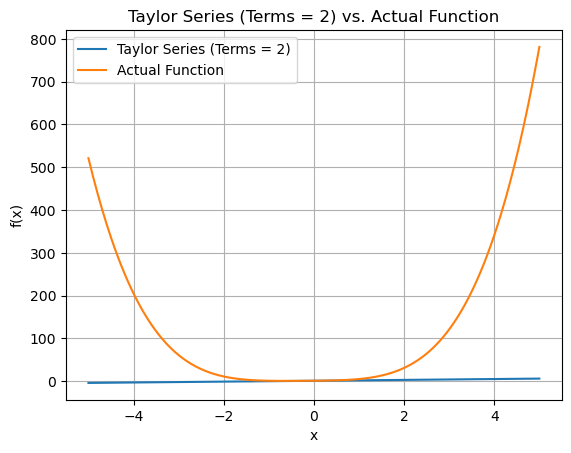 

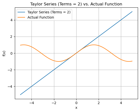
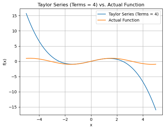
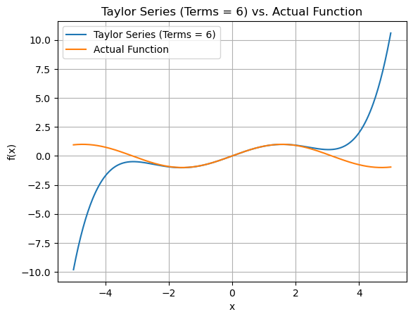
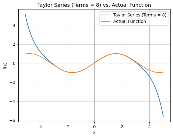
Plotting the graphs for Sin(x)

def function(x):
    return np.sin(x)

x_values = np.linspace(-5, 5, 400)
a = 0

for terms in range(2,10,2):
    plt.figure()
    approx_y_values = [estimate(terms, a, x) for x in x_values]
    plt.plot(x_values, approx_y_values, label=f'Taylor Series (Terms = {terms})')
    plt.plot(x_values, function(x_values), label='Actual Function')
    plt.title(f"Taylor Series (Terms = {terms}) vs. Actual Function")
    plt.xlabel("x")
    plt.ylabel("f(x)")
    plt.legend()
    plt.grid(True)
    plt.show()