Maclaurin Series

The Maclaurin series is a special case of a Taylor series expansion, centered at the origin (x = 0).

\[ e^x = 1 + x + \frac{{x^2}}{2!} + \frac{{x^3}}{3!} + \ldots \]

Import Libraries

import numpy as np
import matplotlib.pyplot as plt

Factorial

\[ x! = x \times (x-1) \times (x-2) \times \ldots \times 3 \times 2 \times 1 \]

def factorial(x):
    if x<=1:
        return 1
    else:
        product=1
        for i in range(1,x+1):
            product*=i
        return product

Let x = 0.5

x=0.5

Exact Ans

exact=np.exp(x)

Estimated Answers

def estimate(terms,x):
    sum = 0
    for i in range(terms+1):
        sum += i*(x**(i-1))/factorial(i)
    return sum

Errors for each term ->

terms = []
errors = []

print("Terms\tExact\t\tEstimate\tError (%)")
print("-------------------------------------------------------")
for i in range(1,11):
    estimate_ans=estimate(i,x)
    error=(exact-estimate_ans)/exact*100
    print(f"{i}\t{exact:.9f}\t{estimate_ans:.9f}\t{error:.9f}%")
    terms.append(i)
    errors.append(error)

plt.figure(figsize=(5, 3))
plt.plot(terms, errors, marker='o')
plt.xlabel("Number of Terms")
plt.ylabel("Error (%)")
plt.title("Error vs. Number of Terms")
plt.grid(True)
plt.show()

Terms   Exact       Estimate    Error (%)
-------------------------------------------------------
1   1.648721271 1.000000000 39.346934029%
2   1.648721271 1.500000000 9.020401043%
3   1.648721271 1.625000000 1.438767797%
4   1.648721271 1.645833333 0.175162256%
5   1.648721271 1.648437500 0.017211563%
6   1.648721271 1.648697917 0.001416494%
7   1.648721271 1.648719618 0.000100238%
8   1.648721271 1.648721168 0.000006220%
9   1.648721271 1.648721265 0.000000344%
10  1.648721271 1.648721270 0.000000017%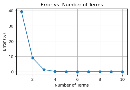

Let x = 5

x=5

Exact Ans

exact=np.exp(x)

Estimated Answers

def estimate(terms,x):
    sum = 0
    for i in range(terms+1):
        sum += i*(x**(i-1))/factorial(i)
    return sum

Errors for each term ->

terms = []
errors = []

print("Terms\tExact\t\tEstimate\tError (%)")
print("-------------------------------------------------------")
for i in range(1,11):
    estimate_ans=estimate(i,x)
    error=(exact-estimate_ans)/exact*100
    print(f"{i}\t{exact:.9f}\t{estimate_ans:.9f}\t{error:.9f}%")
    terms.append(i)
    errors.append(error)

plt.figure(figsize=(5, 3))
plt.plot(terms, errors, marker='o')
plt.xlabel("Number of Terms")
plt.ylabel("Error (%)")
plt.title("Error vs. Number of Terms")
plt.grid(True)
plt.show()

Terms   Exact       Estimate    Error (%)
-------------------------------------------------------
1   148.413159103   1.000000000 99.326205300%
2   148.413159103   6.000000000 95.957231801%
3   148.413159103   18.500000000    87.534798052%
4   148.413159103   39.333333333    73.497408470%
5   148.413159103   65.375000000    55.950671493%
6   148.413159103   91.416666667    38.403934517%
7   148.413159103   113.118055556   23.781653703%
8   148.413159103   128.619047619   13.337167407%
9   148.413159103   138.307167659   6.809363472%
10  148.413159103   143.689456570   3.182805731%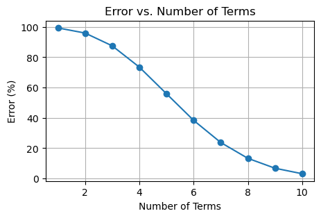

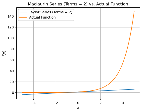
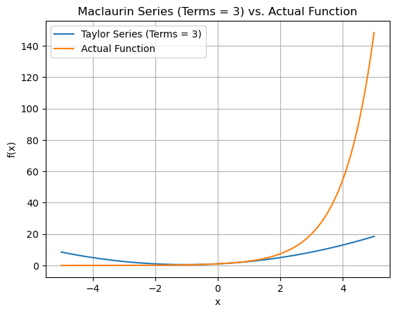
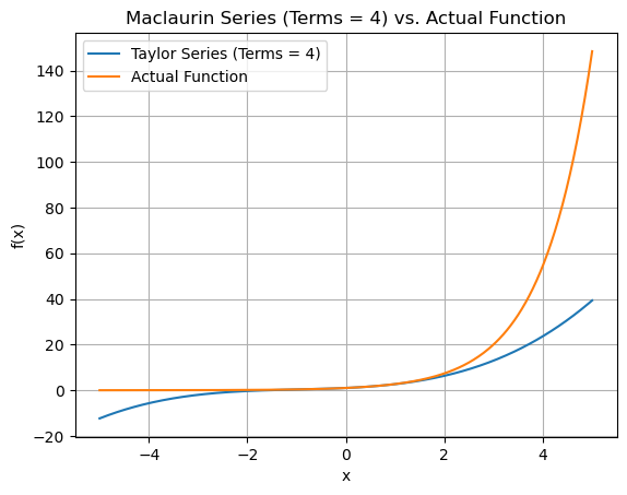
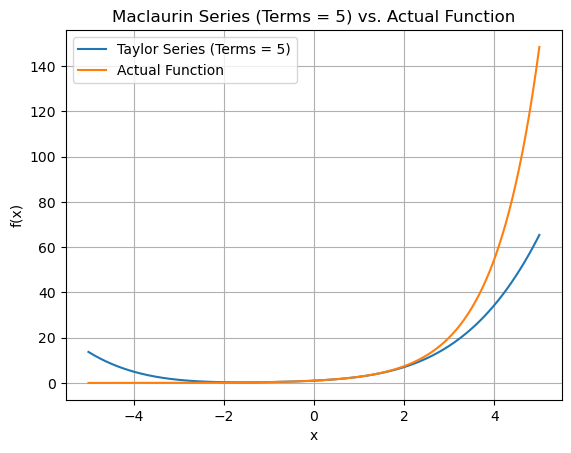
Plotting the graph

x_vals = np.linspace(-5, 5, 400)
exact_vals = np.exp(x_vals)

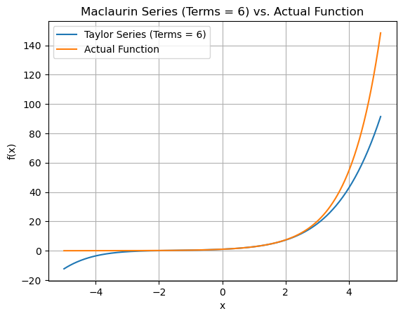
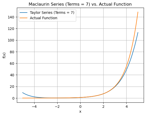
for terms in range(2,8):
    plt.figure()
    approx_y_values = [estimate(terms, x) for x in x_vals]
    plt.plot(x_vals, approx_y_values, label=f'Taylor Series (Terms = {terms})')
    plt.plot(x_vals, exact_vals, label='Actual Function')
    plt.title(f"Maclaurin Series (Terms = {terms}) vs. Actual Function")
    plt.xlabel("x")
    plt.ylabel("f(x)")
    plt.legend()
    plt.grid(True)
    plt.show()