Euler’s Method

Euler’s method is a simple numerical technique used to approximate the solutions of ordinary differential equations (ODEs). It works by iteratively calculating the values of a function at discrete time steps.

Import Libraries

import numpy as np
import matplotlib.pyplot as plt

Exact Equation

Define the Equation

\[\large v = \frac{m \cdot g}{c} \cdot \left( 1 - e^{\large -\frac{ \large c \cdot t}{\large m}}\right) \]

def eqn(t, m, g, c):
    v = (m*g/c)*(1-np.exp(-c*t/m))
    return v

Generate x values

x = np.linspace(0, 40, 400)

Constants

m=80    #(Mass = 80 Kg)
g=9.81  #(Gravitational Const. = 9.81 m/s^2)
c=12.5  #(Drag Coeff. = 12.5 Kg/s)
v_0=0   #(Given that at t=0, v=0)

Calculate y values

y = eqn(x, m, g, c)

Plotting the Exact Function

plt.plot(x, y)
plt.xlabel('t')
plt.ylabel('v')
plt.title('Plot of Exact Equation')
plt.grid(True)
plt.show()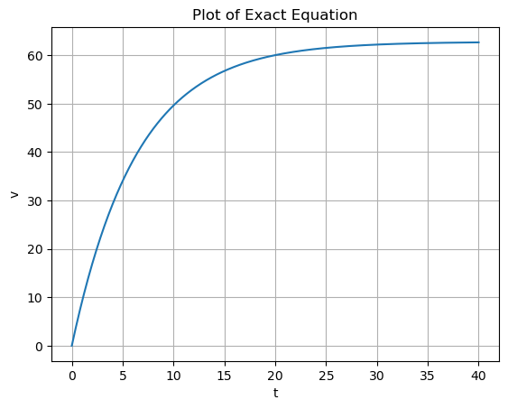

Euler’s Method

\[ \large f(t + h) = f(t) + h \cdot f'(t) \]

Define Differential Eqn

def differential_eqn(v,t):
    return g-c*v/m

Generate x values with step size

step=1
x_e = np.linspace(0, 40, int(40/step))

Calculate y values

y_e=np.zeros(len(x_e))
y_e[0]=v_0

for i in range(len(x_e)-1):
    y_e[i+1]=y_e[i]+differential_eqn(y_e[i],x_e)*step

Plotting the Estimated Function

plt.plot(x_e, y_e)
plt.xlabel('t')
plt.ylabel('v')
plt.title('Plot of Estimated Equation')
plt.grid(True)
plt.show()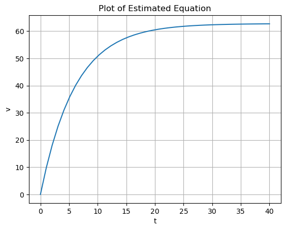

Calculating the error

plt.plot(x_e, y_e, label="Solving by Euler's Eqn")
plt.plot(x, y, label="Solving by Exact Eqn")
plt.title('Plot of Exact and Estimated Equation')
plt.legend()
plt.show()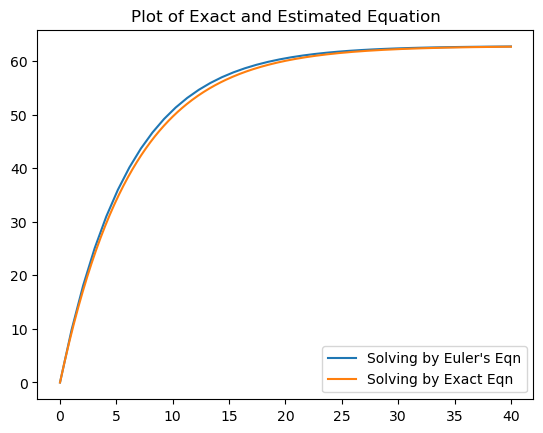

y1=y[::10]+1e-15 

absolute_error = np.abs(y1 - y_e)
percentage_error = (absolute_error / y1) * 100
average_percentage_error = np.mean(percentage_error)

print("Average Percentage Error:", average_percentage_error, "%")

Average Percentage Error: 4.475024083304925 %