Polynomial Regression

Polynomial Regression is a regression technique that models the relationship between a dependent variable and one or more independent variables by fitting a polynomial equation. It expands on linear regression by introducing higher-degree polynomial terms, allowing for a more flexible curve to capture non-linear patterns in the data.

Libraries Required

import numpy as np
import matplotlib.pyplot as plt
import math

Polynomial Features

def create_polynomial_features(X, degree):
    X_poly = np.ones((X.shape[0], 1))
    for d in range(1, degree + 1):
        X_poly = np.hstack((X_poly, X.reshape(-1, 1) ** d))
    return X_poly

def solve_normal_equation(X, y):
    return np.linalg.inv(X.T @ X) @ X.T @ y

def predict(X, coefficients):
    return X @ coefficients

Dataset ( y = 1 + x^2 )

x = np.arange(0, 20, 1)
y = 1 + x**2

plt.scatter(x, y, marker='x', c='r', label="Actual Value")
plt.legend()
plt.title("y=1+x^2")
plt.show()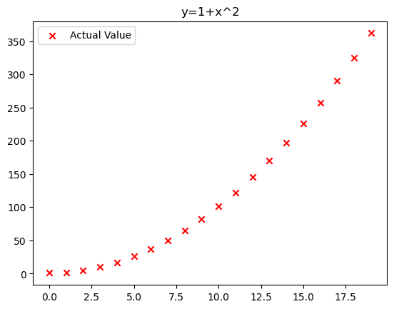

Predictions for Different Degrees

Degree = 0

degree = 0

X_poly = create_polynomial_features(x, degree)

coefficients = solve_normal_equation(X_poly, y)

y_pred = predict(X_poly, coefficients)

# Plot the results
plt.figure(figsize=(12, 6))
plt.scatter(x, y, color='gray', label='Actual')
plt.plot(x, y_pred, color='blue', label='Train Prediction')
plt.xlabel('X')
plt.ylabel('y')
plt.legend()
plt.show()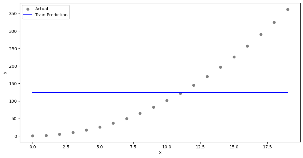

Degree = 1

degree = 1

X_poly = create_polynomial_features(x, degree)

coefficients = solve_normal_equation(X_poly, y)

y_pred = predict(X_poly, coefficients)

# Plot the results
plt.figure(figsize=(12, 6))
plt.scatter(x, y, color='gray', label='Actual')
plt.plot(x, y_pred, color='blue', label='Train Prediction')
plt.xlabel('X')
plt.ylabel('y')
plt.legend()
plt.show()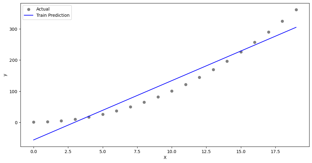

Degree = 2

degree = 2

X_poly = create_polynomial_features(x, degree)

coefficients = solve_normal_equation(X_poly, y)

y_pred = predict(X_poly, coefficients)

# Plot the results
plt.figure(figsize=(12, 6))
plt.scatter(x, y, color='gray', label='Actual')
plt.plot(x, y_pred, color='blue', label='Train Prediction')
plt.xlabel('X')
plt.ylabel('y')
plt.legend()
plt.show()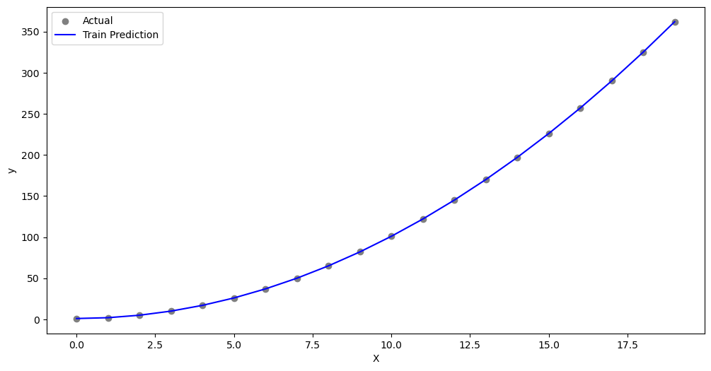

Dataset 2 ( y = Cos(x/2) )

x = np.arange(0,20,1)
y = np.cos(x/2)

plt.scatter(x, y, marker='x', c='r', label="Actual Value")
plt.legend()
plt.title("y=Cos(x/2)")
plt.show()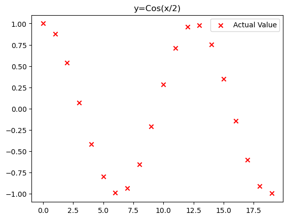

Predictions for Different Degrees

Degree = 1

degree = 1

X_poly = create_polynomial_features(x, degree)

coefficients = solve_normal_equation(X_poly, y)

y_pred = predict(X_poly, coefficients)

# Plot the results
plt.figure(figsize=(12, 6))
plt.scatter(x, y, color='gray', label='Actual')
plt.plot(x, y_pred, color='blue', label='Train Prediction')
plt.xlabel('X')
plt.ylabel('y')
plt.legend()
plt.show()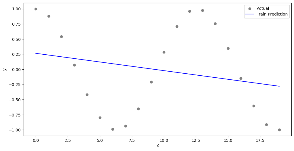

Degree = 4

degree = 4

X_poly = create_polynomial_features(x, degree)

coefficients = solve_normal_equation(X_poly, y)

y_pred = predict(X_poly, coefficients)

# Plot the results
plt.figure(figsize=(12, 6))
plt.scatter(x, y, color='gray', label='Actual')
plt.plot(x, y_pred, color='blue', label='Train Prediction')
plt.xlabel('X')
plt.ylabel('y')
plt.legend()
plt.show()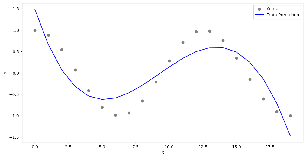

Degree = 9

degree = 9

X_poly = create_polynomial_features(x, degree)

coefficients = solve_normal_equation(X_poly, y)

y_pred = predict(X_poly, coefficients)

# Plot the results
plt.figure(figsize=(12, 6))
plt.scatter(x, y, color='gray', label='Actual')
plt.plot(x, y_pred, color='blue', label='Train Prediction')
plt.xlabel('X')
plt.ylabel('y')
plt.legend()
plt.show()