Logistic Regression

Logistic regression is a statistical tool for understanding the probability of an event occurring based on input variables. It estimates the likelihood using a logistic curve, making it valuable for classification tasks like predicting outcomes or determining categories.

Libraries Required

import numpy as np
import matplotlib.pyplot as plt
import math
from matplotlib import cm

Some Plotting Fxn

def soup_bowl(x_train, y_train, w, b):
    wx, by = np.meshgrid(np.linspace(-6, 12, 50),
                         np.linspace(10, -20, 40))
    points = np.c_[wx.ravel(), by.ravel()]
    cost = np.zeros(points.shape[0])

    for i in range(points.shape[0]):
        w_i, b_i = points[i]
        cost[i] = cost_fxn(x_train, y_train, w_i, b_i)

    cost = cost.reshape(wx.shape)

    fig = plt.figure(figsize=(8, 8))
    ax = fig.add_subplot(1, 1, 1, projection='3d')
    ax.plot_surface(wx, by, cost, alpha=0.6, cmap=cm.jet)
    ax.set_xlabel('w', fontsize=20)
    ax.set_ylabel('b', fontsize=20)
    ax.set_zlabel("Cost", rotation=90, fontsize=20)
    ax.set_title('"Logistic" Squared Error Cost vs (w, b)', fontsize=20)
    cscat = ax.scatter(w, b, s=100, color='red')
    plt.tight_layout()

    plt.show()

Dataset

x_train = np.array([0, 1, 2, 3, 4, 5]).reshape(-1, 1)
y_train = np.array([0,  0, 0, 1, 1, 1])

w = np.array([5])
b = 10

pos = y_train == 1
neg = y_train == 0

plt.figure(figsize=(6, 4))

plt.scatter(x_train[pos], y_train[pos],
            marker='x', s=80, c='red', label="y=1")
plt.scatter(x_train[neg], y_train[neg], marker='o',
            s=100, label="y=0", facecolors='blue', edgecolors='black', linewidth=1)
plt.ylim(-0.08, 1.1)
plt.ylabel('y', fontsize=12)
plt.xlabel('x', fontsize=12)
plt.legend()

plt.tight_layout()
plt.show()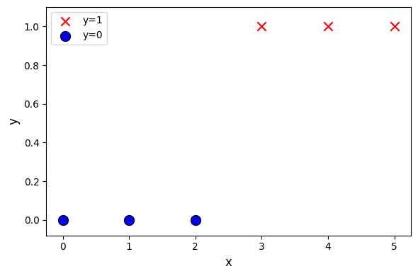

Sigmoid Fxn

\[g(z) = \frac{1}{1+e^{-z}}\]

def sigmoid(x):
    return 1 / (1 + np.exp(-x))


z = np.linspace(-8, 8, 100)

sigmoid_values = sigmoid(z)

plt.figure(figsize=(6, 4))
plt.plot(z, sigmoid_values, label='Sigmoid Function')
plt.xlabel('z')
plt.ylabel('sigmoid(z)')
plt.legend()
plt.grid(True)
plt.show()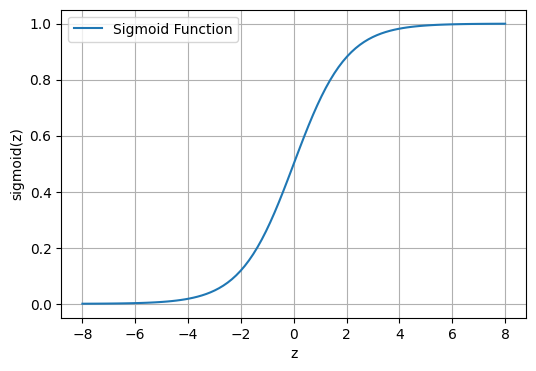

Finding Function f_wb

\[ f_{\mathbf{w},b}(\mathbf{x}^{(i)}) = g(\mathbf{w} \cdot \mathbf{x}^{(i)} + b ) \]

def fxn(x, w, b):
    f_wb = sigmoid(np.dot(x, w) + b)
    return f_wb

Decision Boundary

\[\mathbf{w} \cdot \mathbf{x} = w_0 x_0 + w_1 x_1 = 0\]

Dataset

x_db = np.array([[0.5, 1.5], [1, 1], [1.5, 0.5], [3, 0.5], [2, 2], [1, 2.5]])
y_db = np.array([0, 0, 0, 1, 1, 1]).reshape(-1, 1)

x0 = np.arange(0, 6)

x1 = 3 - x0
fig, ax = plt.subplots(1, 1, figsize=(5, 4))
ax.plot(x0, x1, c="b")
ax.axis([0, 4, 0, 3.5])

ax.fill_between(x0, x1, alpha=0.2)

pos = y_db == 1
neg = y_db == 0
pos = pos.reshape(-1,)
neg = neg.reshape(-1,)

plt.scatter(x_db[neg, 0], x_db[neg, 1], marker='o', s=80,
            label="neg_label", facecolors='none', edgecolors="blue", lw=3)
plt.scatter(x_db[pos, 0], x_db[pos, 1], marker='x',
            s=80, c='red', label="pos_label")
plt.show()
plt.show()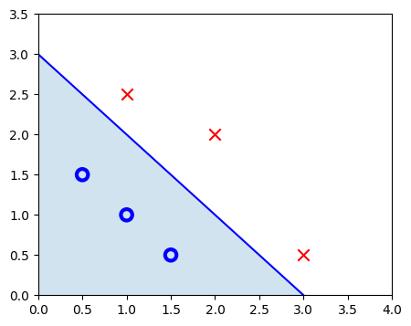

Loss Fxn

\[ loss(f_{\mathbf{w},b}(\mathbf{x}^{(i)}), y^{(i)}) = \begin{cases} - \log\left(f_{\mathbf{w},b}\left( \mathbf{x}^{(i)} \right) \right) & \text{if $y^{(i)}=1$}\\ - \log \left( 1 - f_{\mathbf{w},b}\left( \mathbf{x}^{(i)} \right) \right) & \text{if $y^{(i)}=0$} \end{cases} \]

\[= -y^{(i)} \log\left(f_{\mathbf{w},b}\left( \mathbf{x}^{(i)} \right) \right) - \left( 1 - y^{(i)}\right) \log \left( 1 - f_{\mathbf{w},b}\left( \mathbf{x}^{(i)} \right) \right)\]

def loss(x, y, w, b):
    a = fxn(x, w, b)
    epsilon = 1e-15  # Small constant to avoid taking log(0)

    loss = -y * math.log(a + epsilon) - (1 - y) * math.log(1 - a + epsilon)
    return loss

Cost Fxn

\[ J(\mathbf{w},b) = \frac{1}{m} \sum_{i=0}^{m-1} \left[ loss(f_{\mathbf{w},b}(\mathbf{x}^{(i)}), y^{(i)}) \right]\]

def cost_fxn(X, y, w, b):

    m = X.shape[0]
    cost = 0
    for i in range(m):
        cost += loss(X[i], y[i], w, b)

    cost = cost / m
    return cost

Some Plots ->

Final w, b

if len(w) == 1:
    fxn1 = fxn(x_train, w, b)

    plt.scatter(x_train, y_train, color="red")
    plt.plot(x_train, fxn1)
    plt.show()

soup_bowl(x_train, y_train, w, b)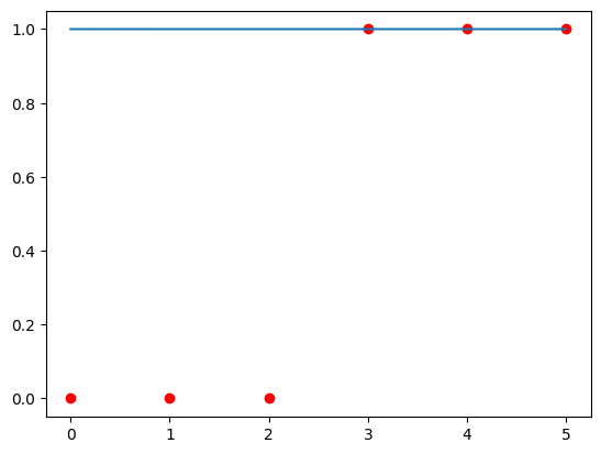

C:\Users\vrajs\AppData\Local\Temp\ipykernel_16560\2055154098.py:5: DeprecationWarning: Conversion of an array with ndim > 0 to a scalar is deprecated, and will error in future. Ensure you extract a single element from your array before performing this operation. (Deprecated NumPy 1.25.)
  loss = -y * math.log(a + epsilon) - (1 - y) * math.log(1 - a + epsilon)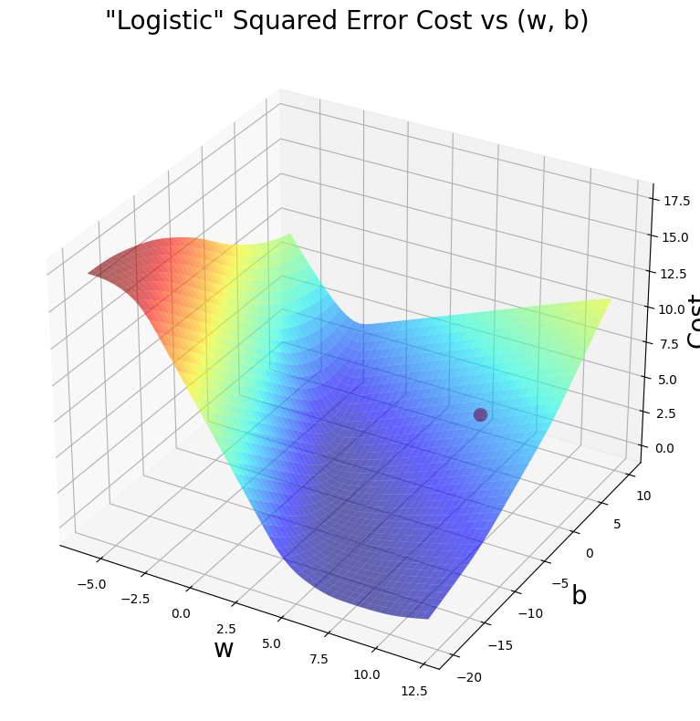

Finding dJ/dw and dJ/db

\[\begin{align*} \frac{\partial J(\mathbf{w},b)}{\partial w_j} &= \frac{1}{m} \sum\limits_{i = 0}^{m-1} (f_{\mathbf{w},b}(\mathbf{x}^{(i)}) - y^{(i)})x_{j}^{(i)} \\ \frac{\partial J(\mathbf{w},b)}{\partial b} &= \frac{1}{m} \sum\limits_{i = 0}^{m-1} (f_{\mathbf{w},b}(\mathbf{x}^{(i)}) - y^{(i)}) \end{align*}\]

def compute_gradient(x, y, w, b):
    dj_dw = 0
    dj_db = 0
    m = x.shape[0]
    a = fxn(x, w, b) - y
    dj_dw = (np.dot(a, x)) / m
    dj_db = np.sum(a) / m
    return dj_dw, dj_db

Gradient Descent

\[\begin{align*} &\text{repeat until convergence:} \; \lbrace \\ & \; \; \;w_j = w_j - \alpha \frac{\partial J(\mathbf{w},b)}{\partial w_j} \; & \text{for j := 0..n-1} \\ & \; \; \; \; \;b = b - \alpha \frac{\partial J(\mathbf{w},b)}{\partial b} \\ &\rbrace \end{align*}\]

def gradient_descent(x, y, w, b, alpha, num_iters):
    J_history = []
    p_history = []

    for i in range(num_iters+1):
        dj_dw, dj_db = compute_gradient(x, y, w, b)
        b = b - alpha * dj_db
        w = w - alpha * dj_dw
        J_history.append(cost_fxn(x, y, w, b))
        p_history.append([w, b])
        if i % math.ceil(num_iters/10) == 0:
            print(f"Iteration {i:4}: Cost {J_history[-1]:0.2e}, w: {w}, b:{b}")

    return w, b, J_history, p_history


iterations = 10000
tmp_alpha = 1.0e-1


w_final, b_final, J_hist, p_hist = gradient_descent(
    x_train, y_train, w, b, tmp_alpha, iterations)
print(f"(w,b) found by gradient descent: ({w_final},{b_final})")


f_wb = fxn(x_train, w_final, b_final)
print("Cost is", cost_fxn(x_train, y_train, w_final, b_final))

Iteration    0: Cost 7.45e+00, w: [4.95000001], b:9.950000761764102
Iteration 1000: Cost 1.32e-01, w: [1.94357846], b:-4.532187811486597
Iteration 2000: Cost 8.42e-02, w: [2.71585819], b:-6.535471646001672
Iteration 3000: Cost 6.46e-02, w: [3.22521954], b:-7.834466336781398
Iteration 4000: Cost 5.30e-02, w: [3.62055449], b:-8.83606124058392
Iteration 5000: Cost 4.51e-02, w: [3.94791911], b:-9.662597001748475
Iteration 6000: Cost 3.92e-02, w: [4.22882495], b:-10.37034842110977
Iteration 7000: Cost 3.48e-02, w: [4.47546538], b:-10.990900553853033
Iteration 8000: Cost 3.12e-02, w: [4.69557844], b:-11.544161480692926
Iteration 9000: Cost 2.83e-02, w: [4.89444965], b:-12.043663029887693
Iteration 10000: Cost 2.59e-02, w: [5.07588043], b:-12.499101969930441
(w,b) found by gradient descent: ([5.07588043],-12.499101969930441)
Cost is 0.025934093960807036

Some Plots ->

Final w, b

if len(w) == 1:
    fxn2 = fxn(x_train, w_final, b_final)

    plt.scatter(x_train, y_train, color="red")
    plt.plot(x_train, fxn2)
    plt.show()
    
soup_bowl(x_train, y_train, w_final, b_final)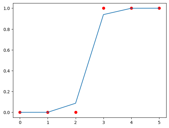

C:\Users\vrajs\AppData\Local\Temp\ipykernel_16560\2055154098.py:5: DeprecationWarning: Conversion of an array with ndim > 0 to a scalar is deprecated, and will error in future. Ensure you extract a single element from your array before performing this operation. (Deprecated NumPy 1.25.)
  loss = -y * math.log(a + epsilon) - (1 - y) * math.log(1 - a + epsilon)

Regularized Linear Regression

Finding Cost Fxn

\[J(\mathbf{w},b) = \frac{1}{2m} \sum\limits_{i = 0}^{m-1} (f_{\mathbf{w},b}(\mathbf{x}^{(i)}) - y^{(i)})^2 + \frac{\lambda}{2m} \sum_{j=0}^{n-1} w_j^2 \]

def cost_fxn_regularized(X, y, w, b, lambda_ = 1):
    cost=cost_fxn(X, y, w, b)
    cost += np.sum(w ** 2)
    return cost

Finding dJ/dw and dJ/db

\[\begin{align*} \frac{\partial J(\mathbf{w},b)}{\partial w_j} &= \frac{1}{m} \sum\limits_{i = 0}^{m-1} (f_{\mathbf{w},b}(\mathbf{x}^{(i)}) - y^{(i)})x_{j}^{(i)} + \frac{\lambda}{m} w_j \\ \frac{\partial J(\mathbf{w},b)}{\partial b} &= \frac{1}{m} \sum\limits_{i = 0}^{m-1} (f_{\mathbf{w},b}(\mathbf{x}^{(i)}) - y^{(i)}) \end{align*}\]

def compute_gradient_regularized(X, y, w, b, lambda_):
    m = X.shape[0]
    dj_dw, dj_db = compute_gradient(X, y, w, b)

    dj_dw += (lambda_ / m) * w

    return dj_db, dj_dw